Hyperalignment for between-subject analysis
Multivariate pattern analysis (MVPA) reveals how the brain represents fine-scale information. Its power lies in its sensitivity to subtle pattern variations that encode this fine-scale information but that also presents a hurdle for group analyses due to between-subject variability of both anatomical & functional architectures. Haxby et al. (2011) recently proposed a method of aligning subjects’ brain data in a high-dimensional functional space and showed how to build a common model of ventral temporal cortex that captures visual object category information. They tested their model by successfully performing between-subject classification of category information. Moreover, when they built the model using a complex naturalistic stimulation (a feature film), it even generalized to other independent experiments even after removing any occurrences of the experimental stimuli from the movie data.
In this example we show how to perform Hyperalignment within a single experiment. We will compare between-subject classification after hyperalignment to between-subject classification on anatomically aligned data (currently the most typical approach), and within-subject classification performance.
Analysis setup
from mvpa2.suite import *

verbose.level = 2
We start by loading preprocessed datasets of 10 subjects with BOLD-responses of stimulation with face and object images (Haxby et al., 2011). Each dataset, after preprocessing, has one sample per category and run for each of the eight runs and seven stimulus categories. Individual subject brains have been aligned anatomically using a 12 dof linear transformation.
verbose(1, "Loading data...")
filepath = os.path.join(cfg.get('location', 'tutorial data'),
                        'hyperalignment_tutorial_data.hdf5.gz')
ds_all = h5load(filepath)
# zscore all datasets individually
_ = [zscore(ds) for ds in ds_all]
# inject the subject ID into all datasets
for i,sd in enumerate(ds_all):
    sd.sa['subject'] = np.repeat(i, len(sd))
# number of subjects
nsubjs = len(ds_all)
# number of categories
ncats = len(ds_all[0].UT)
# number of run
nruns = len(ds_all[0].UC)
verbose(2, "%d subjects" % len(ds_all))
verbose(2, "Per-subject dataset: %i samples with %i features" % ds_all[0].shape)
verbose(2, "Stimulus categories: %s" % ', '.join(ds_all[0].UT))
Now we’ll create a couple of building blocks for the intended analyses. We’ll
use a linear SVM classifier, and perform feature selection with a simple one-way
ANOVA selecting the nf highest scoring features.
# use same classifier
clf = LinearCSVMC()

# feature selection helpers
nf = 100
fselector = FixedNElementTailSelector(nf, tail='upper',
                                      mode='select',sort=False)
sbfs = SensitivityBasedFeatureSelection(OneWayAnova(), fselector,
                                        enable_ca=['sensitivities'])
# create classifier with automatic feature selection
fsclf = FeatureSelectionClassifier(clf, sbfs)
Within-subject classification
We start off by running a cross-validated classification analysis for every subject’s dataset individually. Data folding will be performed by leaving out one run to serve as the testing dataset. ANOVA-based features selection will be performed automatically on training dataset and applied to testing dataset.
verbose(1, "Performing classification analyses...")
verbose(2, "within-subject...", cr=False, lf=False)
wsc_start_time = time.time()
cv = CrossValidation(fsclf,
                     NFoldPartitioner(attr='chunks'),
                     errorfx=mean_match_accuracy)
# store results in a sequence
wsc_results = [cv(sd) for sd in ds_all]
wsc_results = vstack(wsc_results)
verbose(2, " done in %.1f seconds" % (time.time() - wsc_start_time,))
Between-subject classification using anatomically aligned data
For between-subject classification with MNI-aligned voxels, we can stack up all individual datasets into a single one, as (anatomical!) feature correspondence is given. The crossvalidation analysis using the feature selection classifier will automatically perform the desired ANOVA-based feature selection on every training dataset partition. However, data folding will now be done by leaving out a complete subject for testing.
verbose(2, "between-subject (anatomically aligned)...", cr=False, lf=False)
ds_mni = vstack(ds_all)
mni_start_time = time.time()
cv = CrossValidation(fsclf,
                     NFoldPartitioner(attr='subject'),
                     errorfx=mean_match_accuracy)
bsc_mni_results = cv(ds_mni)
verbose(2, "done in %.1f seconds" % (time.time() - mni_start_time,))
Between-subject classification with Hyperalignment(TM)
Between-subject classification using Hyperalignment is very similar to the previous analysis. However, now we no longer assume feature correspondence (or aren’t satisfied with anatomical alignment anymore). Consequently, we have to transform the individual datasets into a common space before performing the classification analysis. To avoid introducing circularity problems to the analysis, we perform leave-one-run-out data folding manually, and train Hyperalignment only on the training dataset partitions. Subsequently, we will apply the derived transformation to the full datasets, stack them up across individual subjects, as before, and run the classification analysis. ANOVA-based feature selection is done in the same way as before (but also manually).
verbose(2, "between-subject (hyperaligned)...", cr=False, lf=False)
hyper_start_time = time.time()
bsc_hyper_results = []
# same cross-validation over subjects as before
cv = CrossValidation(clf, NFoldPartitioner(attr='subject'),
                     errorfx=mean_match_accuracy)

# leave-one-run-out for hyperalignment training
for test_run in range(nruns):
    # split in training and testing set
    ds_train = [sd[sd.sa.chunks != test_run,:] for sd in ds_all]
    ds_test = [sd[sd.sa.chunks == test_run,:] for sd in ds_all]

    # manual feature selection for every individual dataset in the list
    anova = OneWayAnova()
    fscores = [anova(sd) for sd in ds_train]
    featsels = [StaticFeatureSelection(fselector(fscore)) for fscore in fscores]
    ds_train_fs = [featsels[i].forward(sd) for i, sd in enumerate(ds_train)]


    # Perform hyperalignment on the training data with default parameters.
    # Computing hyperalignment parameters is as simple as calling the
    # hyperalignment object with a list of datasets. All datasets must have the
    # same number of samples and time-locked responses are assumed.
    # Hyperalignment returns a list of mappers corresponding to subjects in the
    # same order as the list of datasets we passed in.


    hyper = Hyperalignment()
    hypmaps = hyper(ds_train_fs)

    # Applying hyperalignment parameters is similar to applying any mapper in
    # PyMVPA. We start by selecting the voxels that we used to derive the
    # hyperalignment parameters. And then apply the hyperalignment parameters
    # by running the test dataset through the forward() function of the mapper.

    ds_test_fs = [featsels[i].forward(sd) for i, sd in enumerate(ds_test)]
    ds_hyper = [ hypmaps[i].forward(sd) for i, sd in enumerate(ds_test_fs)]

    # Now, we have a list of datasets with feature correspondence in a common
    # space derived from the training data. Just as in the between-subject
    # analyses of anatomically aligned data we can stack them all up and run the
    # crossvalidation analysis.

    ds_hyper = vstack(ds_hyper)
    # zscore each subject individually after transformation for optimal
    # performance
    zscore(ds_hyper, chunks_attr='subject')
    res_cv = cv(ds_hyper)
    bsc_hyper_results.append(res_cv)

bsc_hyper_results = hstack(bsc_hyper_results)
verbose(2, "done in %.1f seconds" % (time.time() - hyper_start_time,))
Comparing the results
Performance
First we take a look at the classification performance (or accuracy) of all three analysis approaches.
verbose(1, "Average classification accuracies:")
verbose(2, "within-subject: %.2f +/-%.3f"
        % (np.mean(wsc_results),
           np.std(wsc_results) / np.sqrt(nsubjs - 1)))
verbose(2, "between-subject (anatomically aligned): %.2f +/-%.3f"
        % (np.mean(bsc_mni_results),
           np.std(np.mean(bsc_mni_results, axis=1)) / np.sqrt(nsubjs - 1)))
verbose(2, "between-subject (hyperaligned): %.2f +/-%.3f" \
        % (np.mean(bsc_hyper_results),
           np.std(np.mean(bsc_hyper_results, axis=1)) / np.sqrt(nsubjs - 1)))
The output of this demo looks like this:
Loading data...
 10 subjects
 Per-subject dataset: 56 samples with 3509 features
 Stimulus categories: Chair, DogFace, FemaleFace, House, MaleFace, MonkeyFace, Shoe
Performing classification analyses...
 within-subject... done in 4.3 seconds
 between-subject (anatomically aligned)...done after 3.2 seconds
 between-subject (hyperaligned)...done in 10.5 seconds
Average classification accuracies:
 within-subject: 0.57 +/-0.063
 between-subject (anatomically aligned): 0.42 +/-0.035
 between-subject (hyperaligned): 0.62 +/-0.046
It is obvious that the between-subject classification using anatomically aligned data has significantly worse performance when compared to within-subject classification. Clearly the group classification model is inferior to individual classifiers fitted to a particular subject’s data. However, a group classifier trained on hyperaligned data is performing at least as good as the within-subject classifiers – possibly even slightly better due to the increased size of the training dataset.
Similarity structures
To get a better understanding of how hyperalignment transforms the structure of the data, we compare the similarity structures of the corresponding input datasets of all three analysis above (and one in addition).
These are respectively:
- Average similarity structure of the individual data.
- Similarity structure of the averaged hyperaligned data.
- Average similarity structure of the individual data after hyperalignment.
- Similarity structure of the averaged anatomically-aligned data.
Similarity structure in this case is the correlation matrix of multivariate response patterns for all seven stimulus categories in the datasets. For the sake of simplicity, all similarity structures are computed on the full dataset without data folding.
# feature selection as above
anova = OneWayAnova()
fscores = [anova(sd) for sd in ds_all]
fscores = np.mean(np.asarray(vstack(fscores)), axis=0)
# apply to full datasets
ds_fs = [sd[:,fselector(fscores)] for i,sd in enumerate(ds_all)]
#run hyperalignment on full datasets
hyper = Hyperalignment()
mappers = hyper(ds_fs)
ds_hyper = [ mappers[i].forward(ds_) for i,ds_ in enumerate(ds_fs)]
# similarity of original data samples
sm_orig = [np.corrcoef(
                sd.get_mapped(
                    mean_group_sample(['targets'])).samples)
                        for sd in ds_fs]
# mean across subjects
sm_orig_mean = np.mean(sm_orig, axis=0)
# same individual average but this time for hyperaligned data
sm_hyper_mean = np.mean(
                    [np.corrcoef(
                        sd.get_mapped(mean_group_sample(['targets'])).samples)
                            for sd in ds_hyper], axis=0)
# similarity for averaged hyperaligned data
ds_hyper = vstack(ds_hyper)
sm_hyper = np.corrcoef(ds_hyper.get_mapped(mean_group_sample(['targets'])))
# similarity for averaged anatomically aligned data
ds_fs = vstack(ds_fs)
sm_anat = np.corrcoef(ds_fs.get_mapped(mean_group_sample(['targets'])))
We then plot the respective similarity strucures.
# class labels should be in more meaningful order for visualization
# (human faces, animals faces, objects)
intended_label_order = [2,4,1,5,3,0,6]
labels = ds_all[0].UT
labels = labels[intended_label_order]

pl.figure(figsize=(6,6))
# plot all three similarity structures
for i, sm_t in enumerate((
    (sm_orig_mean, "Average within-subject\nsimilarity"),
    (sm_anat, "Similarity of group average\ndata (anatomically aligned)"),
    (sm_hyper_mean, "Average within-subject\nsimilarity (hyperaligned data)"),
    (sm_hyper, "Similarity of group average\ndata (hyperaligned)"),
                      )):
    sm, title = sm_t
    # reorder matrix columns to match label order
    sm = sm[intended_label_order][:,intended_label_order]
    pl.subplot(2, 2, i+1)
    pl.imshow(sm, vmin=-1.0, vmax=1.0, interpolation='nearest')
    pl.colorbar(shrink=.4, ticks=[-1,0,1])
    pl.title(title, size=12)
    ylim = pl.ylim()
    pl.xticks(range(ncats), labels, size='small', stretch='ultra-condensed',
              rotation=45)
    pl.yticks(range(ncats), labels, size='small', stretch='ultra-condensed',
              rotation=45)
    pl.ylim(ylim)
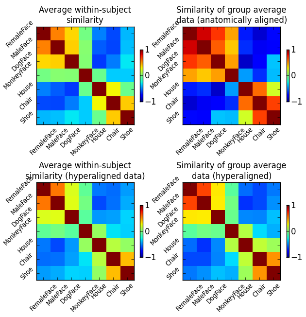
Fig. 1: Correlation of category-specific response patterns using the 100 most informative voxels (based on ANOVA F-score ranking).
We can clearly see that averaging anatomically aligned data has a negative effect on the similarity structure, as the fine category structure is diminished and only the coarse structure (faces vs. objects) is preserved. Moreover, we can see that after hyperalignment the average similarity structure of individual data is essentially identical to the similarity structure of averaged data – reflecting the feature correspondence in the common high-dimensional space.
Regularized Hyperalignment
According to Xu et al. 2012, Hyperalignment can be reformulated to a regularized algorithm that can span the whole continuum between canonical correlation analysis (CCA) and regular hyperalignment by varying a regularization parameter (alpha). Here, we repeat the above between-subject hyperalignment and classification analyses with varying values of alpha from 0 (CCA) to 1.0 (regular hyperalignment).
The following code is essentially identical to the implementation of
between-subject classification shown above. The only difference is an addition
for loop doing the alpha value sweep for each cross-validation fold.
alpha_levels = np.concatenate(
                    (np.linspace(0.0, 0.7, 8),
                     np.linspace(0.8, 1.0, 9)))
# to collect the results for later visualization
bsc_hyper_results = np.zeros((nsubjs, len(alpha_levels), nruns))
# same cross-validation over subjects as before
cv = CrossValidation(clf, NFoldPartitioner(attr='subject'),
                     errorfx=mean_match_accuracy)

# leave-one-run-out for hyperalignment training
for test_run in range(nruns):
    # split in training and testing set
    ds_train = [sd[sd.sa.chunks != test_run,:] for sd in ds_all]
    ds_test = [sd[sd.sa.chunks == test_run,:] for sd in ds_all]

    # manual feature selection for every individual dataset in the list
    anova = OneWayAnova()
    fscores = [anova(sd) for sd in ds_train]
    featsels = [StaticFeatureSelection(fselector(fscore)) for fscore in fscores]
    ds_train_fs = [featsels[i].forward(sd) for i, sd in enumerate(ds_train)]

    for alpha_level, alpha in enumerate(alpha_levels):
        hyper = Hyperalignment(alignment=ProcrusteanMapper(svd='dgesvd',
                                                           space='commonspace'),
                               alpha=alpha)
        hypmaps = hyper(ds_train_fs)
        ds_test_fs = [featsels[i].forward(sd) for i, sd in enumerate(ds_test)]
        ds_hyper = [ hypmaps[i].forward(sd) for i, sd in enumerate(ds_test_fs)]
        ds_hyper = vstack(ds_hyper)
        zscore(ds_hyper, chunks_attr='subject')
        res_cv = cv(ds_hyper)
        bsc_hyper_results[:, alpha_level, test_run] = res_cv.samples.T
Now we can plot the classification accuracy as a function of regularization intensity.
bsc_hyper_results = np.mean(bsc_hyper_results, axis=2)
pl.figure()
plot_err_line(bsc_hyper_results, alpha_levels)
pl.xlabel('Regularization parameter: alpha')
pl.ylabel('Average BSC using hyperalignment +/- SEM')
pl.title('Using regularized hyperalignment with varying alpha values')
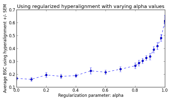
Fig. 2: Mean between-subject classification accuracies using regularized hyperalignment with alpha value ranging from 0 (CCA) to 1 (vanilla hyperalignment).
We can clearly see that the regular hyperalignment performs best for this dataset. However, please refer to Xu et al. 2012 for an example showing that this is not always the case.
See also
The full source code of this example is included in the PyMVPA source distribution (doc/examples/hyperalignment.py).