Analysis of eye movement patterns¶

In this example we are going to look at a classification analysis of eye movement patterns. Although complex preprocessing steps can be performed to extract higher-order features from the raw coordinate timeseries provided by an eye-tracker, we are keeping it simple.

Right after importing the PyMVPA suite, we load the data from a textfile. It contains coordinate timeseries of 144 trials (recorded with 350 Hz), where subjects either looked at upright or inverted images of human faces. Each timeseries snippet covers 3 seconds. This data has been pre-processed to remove eyeblink artefacts.

In addition to the coordinates we also load trial attributes from a second textfile. These attributes indicate which image was shown, whether it was showing a male or female face, and wether it was upright or inverted.

from mvpa2.suite import *

# where is the data
datapath = os.path.join(pymvpa_datadbroot,
                        'face_inversion_demo', 'face_inversion_demo')
# (X, Y, trial id) for all timepoints
data = np.loadtxt(os.path.join(datapath, 'gaze_coords.txt'))
# (orientation, gender, image id) for each trial
attribs = np.loadtxt(os.path.join(datapath, 'trial_attrs.txt'))

As a first step we put the coordinate timeseries into a dataset, and labels each timepoint with its associated trial ID. We also label the two features accordingly.

raw_ds = Dataset(data[:,:2],
                 sa = {'trial': data[:,2]},
                 fa = {'fid': ['rawX', 'rawY']})

The second step is down-sampling the data to about 33 Hz, resampling each trial timeseries individually (using the trial ID attribute to define dataset chunks).

ds = fft_resample(raw_ds, 100, window='hann',
                  chunks_attr='trial', attr_strategy='sample')

Now we can use a BoxcarMapper to turn each trial-timeseries into an individual sample. We know that each sample consists of 100 timepoints. After the dataset is mapped we can add all per-trial attributes into the sample attribute collection.

bm = BoxcarMapper(np.arange(len(ds.sa['trial'].unique)) * 100,
                  boxlength=100)
bm.train(ds)
ds=ds.get_mapped(bm)

ds.sa.update({'orient': attribs[:,0].astype(int),
              'gender': attribs[:,1].astype(int),
              'img_id': attribs[:,1].astype(int)})

In comparison with upright faces, inverted ones had prominent features at very different locations on the screen. Most notably, the eyes were flipped to the bottom half. To prevent the classifier from using such differences, we flip the Y-coordinates for trials with inverted to align the with the upright condition.

ds.samples[ds.sa.orient == 1, :, 1] = \
        -1 * (ds.samples[ds.sa.orient == 1, :, 1] - 512) + 512

The current dataset has 100 two-dimensional features, the X and Y coordinate for each of the hundred timepoints. We use a FlattenMapper to convert each sample into a one-dimensionl vector (of length 200). However, we also keep the original dataset, because it will allow us to perform some plotting much easier.

fm = FlattenMapper()
fm.train(ds)
# want to make a copy to keep the original pristine for later plotting
fds = ds.copy().get_mapped(fm)

# simplify the trial attribute
fds.sa['trial'] = [t[0] for t in ds.sa.trial]

The last steps of preprocessing are Z-scoring all features (coordinate-timepoints) and dividing the dataset into 8 chunks – to simplify a cross-validation analysis.

zscore(fds, chunks_attr=None)

# for classification divide the data into chunks
nchunks =  8
chunks = np.zeros(len(fds), dtype='int')
for o in fds.sa['orient'].unique:
    chunks[fds.sa.orient == o] = np.arange(len(fds.sa.orient == o)) % nchunks
fds.sa['chunks'] = chunks

Now everything is set and we can proceed to the classification analysis. We are using a support vector machine that is going to be trained on the orient attribute, indicating trials with upright and inverted faces. We are going to perform the analysis with a SplitClassifier, because we are also interested in the temporal sensitivity profile. That one is easily accessible via the corresponding sensitivity analyzer.

clf = SVM(space='orient')
mclf = SplitClassifier(clf, space='orient',
                       enable_ca=['confusion'])
sensana = mclf.get_sensitivity_analyzer()
sens = sensana(fds)
print mclf.ca.confusion

The 8-fold cross-validation shows a trial-wise classification accuracy of over 80%. Now we can take a look at the sensitivity. We use the FlattenMapper that is stored in the dataset to unmangle X and Y coordinate vectors in the sensitivity array.

# split mean sensitivities into X and Y coordinate parts by reversing through
# the flatten mapper
xy_sens = fds.a.mapper[-2].reverse(sens).samples

Plotting the results¶

The analysis is done and we can compile a figure to visualize the results. After some inital preparations, we plot an example image of a face that was used in this experiment. We align the image coordinates with the original on-screen coordinates to match them to the gaze track, and overlay the image with the mean gaze track across all trials for each condition.

# descriptive plots
pl.figure()
# original screen size was
axes = ('x', 'y')
screen_size = np.array((1280, 1024))
screen_center = screen_size / 2
colors = ('r','b')
fig = 1

pl.subplot(2, 2, fig)
pl.title('Mean Gaze Track')
face_img = pl.imread(os.path.join(datapath, 'demo_face.png'))
# determine the extend of the image in original screen coordinates
# to match with gaze position
orig_img_extent=(screen_center[0] - face_img.shape[1]/2,
                 screen_center[0] + face_img.shape[1]/2,
                 screen_center[1] + face_img.shape[0]/2,
                 screen_center[1] - face_img.shape[0]/2)
# show face image and put it with original pixel coordinates
pl.imshow(face_img,
          extent=orig_img_extent,
          cmap=pl.cm.gray)
pl.plot(np.mean(ds.samples[ds.sa.orient == 1,:,0], axis=0),
        np.mean(ds.samples[ds.sa.orient == 1,:,1], axis=0),
        colors[0], label='inverted')
pl.plot(np.mean(ds.samples[ds.sa.orient == 2,:,0], axis=0),
        np.mean(ds.samples[ds.sa.orient == 2,:,1], axis=0),
        colors[1], label='upright')
pl.axis(orig_img_extent)
pl.legend()
fig += 1

The next two subplot contain the gaze coordinate over the peri-stimulus time for both, X and Y axis respectively.

pl.subplot(2, 2, fig)
pl.title('Gaze Position X-Coordinate')
plot_erp(ds.samples[ds.sa.orient == 1,:,1], pre=0, errtype = 'std',
         color=colors[0], SR=100./3.)
plot_erp(ds.samples[ds.sa.orient == 2,:,1], pre=0, errtype = 'std',
         color=colors[1], SR=100./3.)
pl.ylim(orig_img_extent[2:])
pl.xlabel('Peristimulus Time')
fig += 1

pl.subplot(2, 2, fig)
pl.title('Gaze Position Y-Coordinate')
plot_erp(ds.samples[ds.sa.orient == 1,:,0], pre=0, errtype = 'std',
         color=colors[0], SR=100./3.)
plot_erp(ds.samples[ds.sa.orient == 2,:,0], pre=0, errtype = 'std',
         color=colors[1], SR=100./3.)
pl.ylim(orig_img_extent[:2])
pl.xlabel('Peristimulus Time')
fig += 1

The last panel has the associated sensitivity profile for both coordinate axes.

pl.subplot(2, 2, fig)
pl.title('SVM-Sensitivity Profiles')
lines = plot_err_line(xy_sens[..., 0], linestyle='-', fmt='ko', errtype='std')
lines[0][0].set_label('X')
lines = plot_err_line(xy_sens[..., 1], linestyle='-', fmt='go', errtype='std')
lines[0][0].set_label('Y')
pl.legend()
pl.ylim((-0.1, 0.1))
pl.xlim(0,100)
pl.axhline(y=0, color='0.6', ls='--')
pl.xlabel('Timepoints')

from mvpa2.base import cfg

The following figure is not exactly identical to the product of this code, but rather shows the result of a few minutes of beautifications in Inkscape.

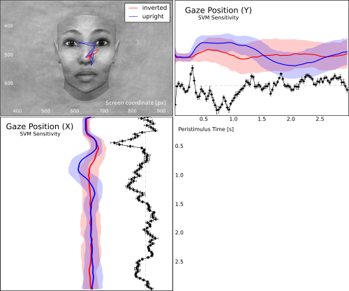
Gaze track for viewing upright vs. inverted faces. The figure shows the mean gaze path for both conditions overlayed on an example face. The panels to the left and below show the X and Y coordinates over the trial timecourse (shaded aread corresponds to one standard deviation across all trials above and below the mean). The black curve depicts the associated temporal SVM weight profile for the classification of both conditions.

Analysis of eye movement patterns¶

Plotting the results¶

Table Of Contents

Previous topic

Next topic