Event-related Data Analysis

Note

This tutorial part is also available for download as an IPython notebook: [ipynb]

In all previous tutorial parts we have analyzed the same fMRI data. We analyzed it using a number of different strategies, but they all had one thing in common: A sample in each dataset was always a single volume from an fMRI time series. Sometimes, we have limited ourselves to just a specific temporal windows of interest, sometimes we averaged many fMRI volumes into a single one. In all cases, however, a feature always corresponded to a voxel in the fMRI volume and appeared only once in the dataset.

In this part we are going to extend the analysis beyond the spatial dimensions and will consider time as another aspect of our data. We will demonstrate two different approaches: 1) modeling of experimental conditions and proceed with an analysis of model parameter estimates, and 2) the extraction of spatio-temporal data samples. The latter approach is common, for example, in ERP-analyses of EEG data.

Let’s start with our well-known example dataset – this time selecting a subset of ventral temporal regions.

>>> from mvpa2.tutorial_suite import *
>>> ds = get_raw_haxby2001_data(roi=(36,38,39,40))

As we know, this dataset consists of 12 concatenated experiment sessions. Every session had a stimulation block spanning multiple fMRI volumes for each of the eight stimulus categories. Stimulation blocks were separated by rest periods.

Event-related Pre-processing Is Not Event-related

For an event-related analysis, most of the processing is done on data samples that are somehow derived from a set of events. The rest of the data could be considered irrelevant. However, some preprocessing is only meaningful when performed on the full time series and not on the segmented event samples. An example is the detrending that typically needs to be done on the original, continuous time series.

In its current shape our datasets consists of samples that represent contiguous fMRI volumes. At this stage we can easily perform linear detrending.

>>> poly_detrend(ds, polyord=1, chunks_attr='chunks')

Let’s make a copy of the de-trended dataset that we can use later on for some visualization.

>>> orig_ds = ds.copy()

Design Specification

For any event-related analysis we need some information on the experiment design: when was stimulated with what for how long (and maybe with what intensity). In PyMVPA this is done by compiling a list of event definitions. In many cases, an event is defined by onset, duration and potentially a number of additional properties, such as stimulus condition or recording session number.

To see how such events definitions look like, we will simply convert the block-design setup defined by the samples attributes of our dataset into a list of events. With find_events(), PyMVPA provides a function to convert sequential attributes into event lists. In our dataset, we have the stimulus conditions of each volume sample available in the targets sample attribute.

>>> events = find_events(targets=ds.sa.targets, chunks=ds.sa.chunks)
>>> print len(events)
204
>>> for e in events[:4]:
...    print e
{'chunks': 0, 'duration': 6, 'onset': 0, 'targets': 'rest'}
{'chunks': 0, 'duration': 9, 'onset': 6, 'targets': 'scissors'}
{'chunks': 0, 'duration': 6, 'onset': 15, 'targets': 'rest'}
{'chunks': 0, 'duration': 9, 'onset': 21, 'targets': 'face'}

We are feeding not only the targets to the function, but also the chunks attribute, since we do not want to have events spanning multiple recording sessions. find_events() sequentially parses all provided attributes and records an event whenever the value in any of the attributes changes. The generated event definition is a dictionary that contains:

1. Onset of the event as an index in the sequence (in this example this is a volume id)
2. Duration of the event in “number of sequence elements” (i.e. number of volumes). The duration is determined by counting the number of identical attribute combinations following an event onset.
3. Attribute combination of this event, i.e. the actual values of all given attributes at the particular position.

Let’s limit ourselves to face and house stimulation blocks for now. We can easily filter out all other events.

>>> events = [ev for ev in events if ev['targets'] in ['house', 'face']]
>>> print len(events)
24
>>> for e in events[:4]:
...    print e
{'chunks': 0, 'duration': 9, 'onset': 21, 'targets': 'face'}
{'chunks': 0, 'duration': 9, 'onset': 63, 'targets': 'house'}
{'chunks': 1, 'duration': 9, 'onset': 127, 'targets': 'face'}
{'chunks': 1, 'duration': 9, 'onset': 213, 'targets': 'house'}

Response Modeling

Whenever we have to deal with data were multiple concurrent signals are overlapping in time, such as in fast event-related fMRI studies, it often makes sense to fit an appropriate model to the data and proceed with an analysis of model parameter estimates, instead of the raw data.

PyMVPA can make use of NiPy’s GLM modeling capabilities. It expects information on stimulation events to be given as actual time stamps and not data sample indices, hence we have to convert our event list.

>>> # temporal distance between samples/volume is the volume repetition time
>>> TR = np.median(np.diff(ds.sa.time_coords))
>>> # convert onsets and durations into timestamps
>>> for ev in events:
...     ev['onset'] = (ev['onset'] * TR)
...     ev['duration'] = ev['duration'] * TR

Now we can fit a model of the hemodynamic response to all relevant stimulus conditions. The function eventrelated_dataset() does everything for us. For a given input dataset we need to provide a list of events, the name of an attribute with a time stamp for each sample, and information on what conditions we would like to have modeled. The latter is specified to the condition_attr argument. This can be a single attribute name in which case all unique values will be used as conditions. It can also be a sequence of multiple attribute names, and all combinations of unique values of the attributes will be used as conditions. In the following example ('targets', 'chunks') indicates that we want a separate model for each stimulation condition (targets) for each run of our example dataset (chunks).

>>> evds = fit_event_hrf_model(ds,
...                            events,
...                            time_attr='time_coords',
...                            condition_attr=('targets', 'chunks'))
>>> print len(evds)
24

This yields one parameter estimate sample for each target value for each chunks.

Exercise

Explore the evds dataset. It contains the generated HRF model. Find and plot (some of) them. Take a look at the parameter estimate samples themselves – can you spot a pattern?

Before we can run a classification analysis we still need to normalize each feature (GLM parameters estimates for each voxel at this point).

>>> zscore(evds, chunks_attr=None)

The rest is straight-forward: we set up a cross-validation analysis with a chosen classifier and run it:

>>> clf = kNN(k=1, dfx=one_minus_correlation, voting='majority')
>>> cv = CrossValidation(clf, NFoldPartitioner(attr='chunks'))
>>> cv_glm = cv(evds)
>>> print '%.2f' % np.mean(cv_glm)
0.04

Not bad! Let’s compare that to a simpler approach that is also suitable for block-design experiments like this one.

>>> zscore(ds, param_est=('targets', ['rest']))
>>> avgds = ds.get_mapped(mean_group_sample(['targets', 'chunks']))
>>> avgds = avgds[np.array([t in ['face', 'house'] for t in avgds.sa.targets])]

We normalize all voxels with respect to the rest condition. This yields some crude kind of “activation” score for all stimulation conditions. Subsequently, we average all sample of a condition in each run. This yield a dataset of the same size as from the GLM modeling. We can re-use the cross-validation setup.

>>> cv_avg = cv(avgds)
>>> print '%.2f' % np.mean(cv_avg)
0.04

Not bad either. However, it is worth repeating that this simple average-sample approach is limited to block-designs with a clear temporal separation of all signals of interest, whereas the HRF modeling is more suitable for experiments with fast stimulation alternation.

Exercise

Think about what need to be done to perform odd/even run GLM modeling.

From Timeseries To Spatio-temporal Samples

Now we want to try something different. Instead of compressing all temporal information into a single model parameter estimate, we can also consider the entire spatio-temporal signal across our region of interest and the full duration of the stimulation blocks. In other words, we can perform a sensitivity analysis (see Classification Model Parameters – Sensitivity Analysis) revealing the spatio-temporal distribution of classification-relevant information.

Before we start with our event-extraction, we want to normalize each feature (i.e. a voxel at this point). In this case we are, again, going to Z-score them, using the mean and standard deviation from the experiment’s rest condition, and the resulting values might be interpreted as “activation scores”.

>>> zscore(ds, chunks_attr='chunks', param_est=('targets', 'rest'))

For this analysis we do not have to convert event onset information into time-stamp, but can operate on sample indices, hence we start with the original event list again.

>>> events = find_events(targets=ds.sa.targets, chunks=ds.sa.chunks)
>>> events = [ev for ev in events if ev['targets'] in ['house', 'face']]

All of our events are of the same length, 9 consecutive fMRI volumes. Later on we would like to view the temporal sensitivity profile from before until after the stimulation block, hence we should extend the duration of the events a bit.

>>> event_duration = 13
>>> for ev in events:
...     ev['onset'] -= 2
...     ev['duration'] = event_duration

The next and most important step is to actually segment the original time series dataset into event-related samples. PyMVPA offers eventrelated_dataset() as a function to perform this conversion. Let’s just do it, it only needs the original dataset and our list of events.

>>> evds = eventrelated_dataset(ds, events=events)
>>> len(evds) == len(events)
True
>>> evds.nfeatures == ds.nfeatures * event_duration
True

Exercise

Inspect the evds dataset. It has a fairly large number of attributes – both for samples and for features. Look at each of them and think about what it could be useful for.

At this point it is worth looking at the dataset’s mapper – in particular at the last two items in the chain mapper that have been added during the conversion into events.

>>> print evds.a.mapper[-2:]
<Chain: <Boxcar: bl=13>-<Flatten>>

Exercise

Reverse-map a single sample through the last two items in the chain mapper. Inspect the result and make sure it doesn’t surprise. Now, reverse-map multiple samples at once and compare the result. Is this what you would expect?

The rest of our analysis is business as usual and is quickly done. We want to perform a cross-validation analysis of an SVM classifier. We are not primarily interested in its performance, but in the weights it assigns to the features. Remember, each feature is now voxel-at-time-point, so we get a chance of looking at the spatio-temporal profile of classification-relevant information in the data. We will nevertheless enable computing of a confusion matrix, so we can assure ourselves that the classifier is performing reasonably well, because only a generalizing model is worth inspecting, as otherwise it overfits and the assigned weights could be meaningless.

>>> sclf = SplitClassifier(LinearCSVMC(),
...                        enable_ca=['stats'])
>>> sensana = sclf.get_sensitivity_analyzer()
>>> sens = sensana(evds)

Exercise

Check that the classifier achieves an acceptable accuracy. Is it enough above chance level to allow for an interpretation of the sensitivities?

Exercise

Using what you have learned in the last tutorial part: Combine the sensitivity maps for all splits into a single map. Project this map into the original dataspace. What is the shape of that space? Store the projected map into a NIfTI file and inspect it using an MRI viewer. Viewer needs to be capable of visualizing time series (hint: for FSLView the time series image has to be opened first)!

A Plotting Example

We have inspected the spatio-temporal profile of the sensitivities using some MRI viewer application, but we can also assemble an informative figure right here. Let’s compose a figure that shows the original peri-stimulus time series, the effect of normalization, as well as the corresponding sensitivity profile of the trained SVM classifier. We are going to do that for two example voxels, whose coordinates we might have derived from inspecting the full map.

>>> example_voxels = [(28,25,25), (28,23,25)]

The plotting will be done by the popular matplotlib package.

First, we plot the original signal after initial detrending. To do this, we apply the same time series segmentation to the original detrended dataset and plot the mean signal for all face and house events for both of our example voxels. The code below will create the plot using matplotlib’s pylab interface (imported as pl). If you are familiar with Matlab’s plotting facilities, this shouldn’t be hard to read.

Note

_ = is used in the examples below simply to absorb output of plotting functions. You do not have to swallow output in your interactive sessions.

>>> # linestyles and colors for plotting
>>> vx_lty = ['-', '--']
>>> t_col = ['b', 'r']
>>>
>>> # for each of the example voxels
>>> for i, v in enumerate(example_voxels):
...     # get a slicing array matching just to current example voxel
...     slicer = np.array([tuple(idx) == v for idx in ds.fa.voxel_indices])
...     # perform the timeseries segmentation just for this voxel
...     evds_detrend = eventrelated_dataset(orig_ds[:, slicer], events=events)
...     # now plot the mean timeseries and standard error
...     for j, t in enumerate(evds.uniquetargets):
...         l = plot_err_line(evds_detrend[evds_detrend.sa.targets == t].samples,
...                           fmt=t_col[j], linestyle=vx_lty[i])
...         # label this plot for automatic legend generation
...         l[0][0].set_label('Voxel %i: %s' % (i, t))
>>> # y-axis caption
>>> _ = pl.ylabel('Detrended signal')
>>> # visualize zero-level
>>> _ = pl.axhline(linestyle='--', color='0.6')
>>> # put automatic legend
>>> _ = pl.legend()
>>> _ = pl.xlim((0,12))

In the next figure we do exactly the same again, but this time for the normalized data.

>>> for i, v in enumerate(example_voxels):
...     slicer = np.array([tuple(idx) == v for idx in ds.fa.voxel_indices])
...     evds_norm = eventrelated_dataset(ds[:, slicer], events=events)
...     for j, t in enumerate(evds.uniquetargets):
...         l = plot_err_line(evds_norm[evds_norm.sa.targets == t].samples,
...                           fmt=t_col[j], linestyle=vx_lty[i])
...         l[0][0].set_label('Voxel %i: %s' % (i, t))
>>> _ = pl.ylabel('Normalized signal')
>>> _ = pl.axhline(linestyle='--', color='0.6')
>>> _ = pl.xlim((0,12))

Finally, we plot the associated SVM weight profile for each peri-stimulus time-point of both voxels. For easier selection we do a little trick and reverse-map the sensitivity profile through the last mapper in the dataset’s chain mapper (look at evds.a.mapper for the whole chain). This will reshape the sensitivities into cross-validation fold x volume x voxel features.

>>> # L1 normalization of sensitivity maps per split to make them
>>> # comparable
>>> normed = sens.get_mapped(FxMapper(axis='features', fx=l1_normed))
>>> smaps = evds.a.mapper[-1].reverse(normed)
>>>
>>> for i, v in enumerate(example_voxels):
...     slicer = np.array([tuple(idx) == v for idx in ds.fa.voxel_indices])
...     smap = smaps.samples[:,:,slicer].squeeze()
...     l = plot_err_line(smap, fmt='ko', linestyle=vx_lty[i], errtype='std')
>>> _ = pl.xlim((0,12))
>>> _ = pl.ylabel('Sensitivity')
>>> _ = pl.axhline(linestyle='--', color='0.6')
>>> _ = pl.xlabel('Peristimulus volumes')

That was it. Perhaps you are scared by the amount of code. Please note that it could have been done shorter, but this way allows for plotting any other voxel coordinate combination as well. matplotlib also allows for saving this figure in SVG format, allowing for convenient post-processing in Inkscape – a publication quality figure is only minutes away.

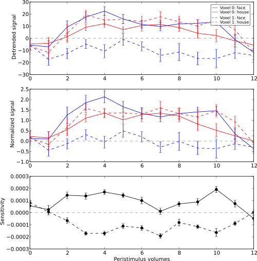
Sensitivity profile for two example voxels for face vs. house classification on event-related fMRI data from ventral temporal cortex.

Exercise

What can we say about the properties of the example voxel’s signal from the peri-stimulus plot?

This demo showed an event-related data analysis. Although we have performed it on fMRI data, an analogous analysis can be done for any time series based data in an almost identical fashion. Moreover, if a dataset has information about acquisition time (e.g. like the ones created by fmri_dataset()) eventrelated_dataset() can also convert event-definition in real time, making it relatively easy to “convert” experiment design logfiles into event lists. In this case there would be no need to run a function like find_events(), but instead they could be directly specified and passed to eventrelated_dataset().