Sensitivity Measure
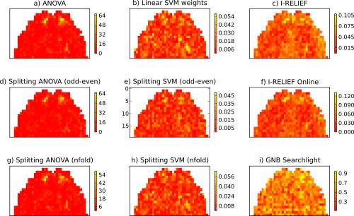
Run some basic and meta sensitivity measures on the example fMRI dataset that comes with PyMVPA and plot the computed featurewise measures for each. The generated figure shows sensitivity maps computed by six sensitivity analyzers.
We start by loading PyMVPA and the example fMRI dataset.
from mvpa2.suite import *

# load PyMVPA example dataset with literal labels
dataset = load_example_fmri_dataset(literal=True)
print dataset.a
As with classifiers it is easy to define a bunch of sensitivity
analyzers. It is usually possible to simply call get_sensitivity_analyzer()
on any classifier to get an instance of an appropriate sensitivity analyzer
that uses this particular classifier to compute and extract sensitivity scores.
# define sensitivity analyzer
sensanas = {
    'a) ANOVA': OneWayAnova(postproc=absolute_features()),
    'b) Linear SVM weights': LinearNuSVMC().get_sensitivity_analyzer(
                                               postproc=absolute_features()),
    'c) I-RELIEF': IterativeRelief(postproc=absolute_features()),
    'd) Splitting ANOVA (odd-even)':
        RepeatedMeasure(
            OneWayAnova(postproc=absolute_features()),
            OddEvenPartitioner()),
    'e) Splitting SVM (odd-even)':
        RepeatedMeasure(
            LinearNuSVMC().get_sensitivity_analyzer(postproc=absolute_features()),
            OddEvenPartitioner()),
    'f) I-RELIEF Online':
        IterativeReliefOnline(postproc=absolute_features()),
    'g) Splitting ANOVA (nfold)':
        RepeatedMeasure(
            OneWayAnova(postproc=absolute_features()),
            NFoldPartitioner()),
    'h) Splitting SVM (nfold)':
        RepeatedMeasure(
            LinearNuSVMC().get_sensitivity_analyzer(postproc=absolute_features()),
            NFoldPartitioner()),
    'i) GNB Searchlight':
        sphere_gnbsearchlight(GNB(), NFoldPartitioner(cvtype=1),
                              radius=0, errorfx=mean_match_accuracy)
           }
Now, we are performing some a more or less standard preprocessing steps: detrending, selecting a subset of the experimental conditions, normalization of each feature to a standard mean and variance.
# do chunkswise linear detrending on dataset
poly_detrend(dataset, polyord=1, chunks_attr='chunks')

# only use 'rest', 'shoe' and 'bottle' samples from dataset
dataset = dataset[np.array([l in ['rest', 'shoe', 'bottle']
                    for l in dataset.sa.targets], dtype='bool')]

# zscore dataset relative to baseline ('rest') mean
zscore(dataset, chunks_attr='chunks',
       param_est=('targets', ['rest']), dtype='float32')

# remove baseline samples from dataset for final analysis
dataset = dataset[dataset.sa.targets != 'rest']
Finally, we will loop over all defined analyzers and let them compute the sensitivity scores. The resulting vectors are then mapped back into the dataspace of the original fMRI samples, which are then plotted.
fig = 0
pl.figure(figsize=(14, 8))

keys = sensanas.keys()
keys.sort()

for s in keys:
    # tell which one we are doing
    print "Running %s ..." % (s)

    sana = sensanas[s]
    # compute sensitivies
    sens = sana(dataset)
    # I-RELIEF assigns zeros, which corrupts voxel masking for pylab's
    # imshow, so adding some epsilon :)
    smap = sens.samples[0] + 0.00001

    # map sensitivity map into original dataspace
    orig_smap = dataset.mapper.reverse1(smap)
    masked_orig_smap = np.ma.masked_array(orig_smap, mask=orig_smap == 0)

    # make a new subplot for each classifier
    fig += 1
    pl.subplot(3, 3, fig)

    pl.title(s)

    pl.imshow(masked_orig_smap[..., 0].T,
             interpolation='nearest',
             aspect=1.25,
             cmap=pl.cm.autumn)

    # uniform scaling per base sensitivity analyzer
    ## if s.count('ANOVA'):
    ##     pl.clim(0, 30)
    ## elif s.count('SVM'):
    ##     pl.clim(0, 0.055)
    ## else:
    ##     pass

    pl.colorbar(shrink=0.6)
Output of the example analysis:
See also
The full source code of this example is included in the PyMVPA source distribution (doc/examples/sensanas.py).