Searchlight on fMRI data
The original idea of a spatial searchlight algorithm stems from a paper by Kriegeskorte et al. (2006), and has subsequently been used in a number of studies. The most common use for a searchlight is to compute a full cross-validation analysis in each spherical region of interest (ROI) in the brain. This analysis yields a map of (typically) classification accuracies that are often interpreted or post-processed similar to a GLM statistics output map (e.g. subsequent analysis with inferential statistics). In this example we look at how this type of analysis can be conducted in PyMVPA.
As always, we first have to import PyMVPA.
from mvpa2.suite import *
As searchlight analyses are usually quite expensive in terms of computational resources, we are going to enable some progress output to entertain us while we are waiting.
# enable debug output for searchlight call
if __debug__:
    debug.active += ["SLC"]
The next few calls load an fMRI dataset, while assigning associated class
targets and chunks (experiment runs) to each volume in the 4D timeseries. One
aspect is worth mentioning. When loading the fMRI data with
fmri_dataset() additional feature attributes can be
added, by providing a dictionary with names and source pairs to the add_fa
arguments. In this case we are loading a thresholded zstat-map of a category
selectivity contrast for voxels ventral temporal cortex.
# data path
datapath = os.path.join(mvpa2.cfg.get('location', 'tutorial data'), 'haxby2001')
dataset = load_tutorial_data(
        roi='brain',
        add_fa={'vt_thr_glm': os.path.join(datapath, 'sub001', 'masks',
                                                     'orig', 'vt.nii.gz')})
The dataset is now loaded and contains all brain voxels as features, and all volumes as samples. To precondition this data for the intended analysis we have to perform a few preprocessing steps (please note that the data was already motion-corrected). The first step is a chunk-wise (run-wise) removal of linear trends, typically caused by the acquisition equipment.
poly_detrend(dataset, polyord=1, chunks_attr='chunks')
Now that the detrending is done, we can remove parts of the timeseries we are not interested in. For this example we are only considering volumes acquired during a stimulation block with images of houses and scrambled pictures, as well as rest periods (for now). It is important to perform the detrending before this selection, as otherwise the equal spacing of fMRI volumes is no longer guaranteed.
dataset = dataset[np.array([l in ['rest', 'house', 'scrambledpix']
                           for l in dataset.targets], dtype='bool')]
The final preprocessing step is data-normalization. This is a required step for many classification algorithms. It scales all features (voxels) into approximately the same range and removes the mean. In this example, we perform a chunk-wise normalization and compute standard deviation and mean for z-scoring based on the volumes corresponding to rest periods in the experiment. The resulting features could be interpreted as being voxel salience relative to ‘rest’.
zscore(dataset, chunks_attr='chunks', param_est=('targets', ['rest']), dtype='float32')
After normalization is completed, we no longer need the ‘rest’-samples and remove them.
dataset = dataset[dataset.sa.targets != 'rest']
But now for the interesting part: Next we define the measure that shall be computed for each sphere. Theoretically, this can be anything, but here we choose to compute a full leave-one-out cross-validation using a linear Nu-SVM classifier.
# choose classifier
clf = LinearNuSVMC()

# setup measure to be computed by Searchlight
# cross-validated mean transfer using an N-fold dataset splitter
cv = CrossValidation(clf, NFoldPartitioner())
In this example, we do not want to compute full-brain accuracy maps, but instead limit ourselves to a specific subset of voxels. We’ll select all voxel that have a non-zero z-stats value in the localizer mask we loaded above, as center coordinates for a searchlight sphere. These spheres will still include voxels that did not pass the threshold. the localizer merely define the location of all to be processed spheres.
# get ids of features that have a nonzero value
center_ids = dataset.fa.vt_thr_glm.nonzero()[0]
Finally, we can run the searchlight. We’ll perform the analysis for three
different radii, each time computing an error for each sphere. To achieve this,
we simply use the sphere_searchlight() class,
which takes any processing object and a radius as arguments. The
processing object has to compute the intended measure, when called with
a dataset. The sphere_searchlight() object
will do nothing more than generate small datasets for each sphere, feeding them
to the processing object, and storing the result.
# setup plotting parameters (not essential for the analysis itself)
plot_args = {
    'background' : os.path.join(datapath, 'sub001', 'anatomy', 'highres001.nii.gz'),
    'background_mask' : os.path.join(datapath, 'sub001', 'masks', 'orig', 'brain.nii.gz'),
    'overlay_mask' : os.path.join(datapath, 'sub001', 'masks', 'orig', 'vt.nii.gz'),
    'do_stretch_colors' : False,
    'cmap_bg' : 'gray',
    'cmap_overlay' : 'autumn', # YlOrRd_r # pl.cm.autumn
    'interactive' : cfg.getboolean('examples', 'interactive', True),
    }

for radius in [0, 1, 3]:
    # tell which one we are doing
    print "Running searchlight with radius: %i ..." % (radius)
Here we actually setup the spherical searchlight by configuring the
radius, and our selection of sphere center coordinates. Moreover, via the
space argument we can instruct the searchlight which feature attribute
shall be used to determine the voxel neighborhood. By default,
fmri_dataset() creates a corresponding attribute
called voxel_indices. Using the mapper argument it is possible to
post-process the results computed for each sphere. Cross-validation will
compute an error value per each fold, but here we are only interested in
the mean error across all folds. Finally, on multi-core machines nproc
can be used to enabled parallelization by setting it to the number of
processes utilized by the searchlight (default value of nproc`=`None utilizes
all available local cores).
»    sl = sphere_searchlight(cv, radius=radius, space='voxel_indices',
                             center_ids=center_ids,
                             postproc=mean_sample())
Since we care about efficiency, we are stripping all attributes from the dataset that are not required for the searchlight analysis. This will offers some speedup, since it reduces the time that is spent on dataset slicing.
»    ds = dataset.copy(deep=False,
                       sa=['targets', 'chunks'],
                       fa=['voxel_indices'],
                       a=['mapper'])
Finally, we actually run the analysis. The result is returned as a dataset. For the upcoming plots, we are transforming the returned error maps into accuracies.
»    sl_map = sl(ds)
     sl_map.samples *= -1
     sl_map.samples += 1
The result dataset is fully aware of the original dataspace. Using this information we can map the 1D accuracy maps back into “brain-space” (using NIfTI image header information from the original input timeseries.
» niftiresults = map2nifti(sl_map, imghdr=dataset.a.imghdr)
PyMVPA comes with a convenient plotting function to visualize the searchlight maps. We are only looking at fMRI slices that are covered by the mask of ventral temproal cortex.
»    fig = pl.figure(figsize=(12, 4), facecolor='white')
     subfig = plot_lightbox(overlay=niftiresults,
                            vlim=(0.5, None), slices=range(23,31),
                            fig=fig, **plot_args)
     pl.title('Accuracy distribution for radius %i' % radius)
The following figures show the resulting accuracy maps for the slices covered by the ventral temporal cortex mask. Note that each voxel value represents the accuracy of a sphere centered around this voxel.
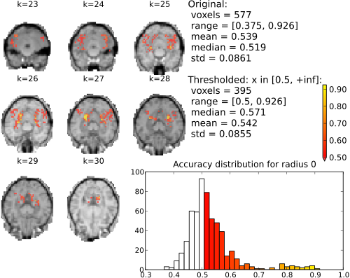
Searchlight (single element; univariate) accuracy maps for binary classification house vs. scrambledpix.
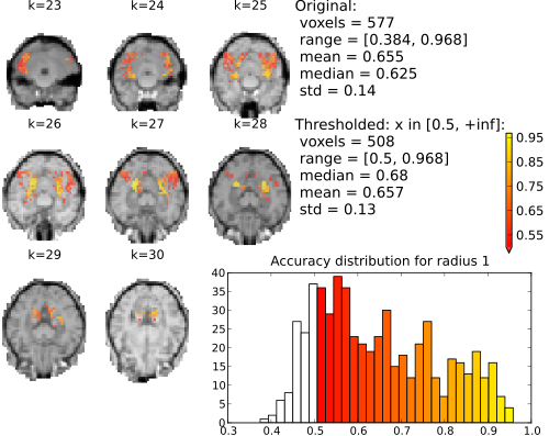
Searchlight (sphere of neighboring voxels; 9 elements) accuracy maps for binary classification house vs. scrambledpix.
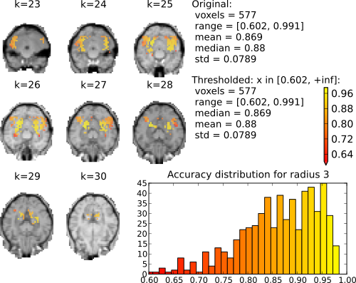
Searchlight (radius 3 elements; 123 voxels) accuracy maps for binary classification house vs. scrambledpix.
With radius 0 (only the center voxel is part of the part the sphere) there is a clear distinction between two distributions. The chance distribution, relatively symetric and centered around the expected chance-performance at 50%. The second distribution, presumambly of voxels with univariate signal, is nicely segregated from that. Increasing the searchlight size significantly blurrs the accuracy map, but also lead to an increase in classification accuracy.
See also
The full source code of this example is included in the PyMVPA source distribution (doc/examples/searchlight.py).