Basic (f)MRI plotting

When running an fMRI data analysis it is often necessary to visualize results in their original dataspace, typically as an overlay on some anatomical brain image. PyMVPA has the ability to export results into the NIfTI format, and via this data format it is compatible with virtually any MRI visualization software.

However, sometimes having a scriptable plotting facility within Python is desired. There are a number of candidate tools for this purpose (e.g. Mayavi), but also PyMVPA itself offers some basic MRI plotting.

In this example, we are showing a quick-and-dirty plot of a voxel-wise ANOVA measure, overlaid on the respective brain anatomy. Note that the plotting is not specific to ANOVAs. Any feature-wise measure can be plotted this way.

We start with basic steps: loading PyMVPA and the example fMRI dataset, only select voxels that correspond to some pre-computed gray matter mask, do basic preprocessing, and estimate ANOVA scores. This has already been described elsewhere, hence we only provide the code here for the sake of completeness.

from mvpa2.suite import *

# load PyMVPA example dataset
datapath = os.path.join(mvpa2.cfg.get('location', 'tutorial data'), 'haxby2001')
dataset = load_tutorial_data(roi='gray')

# do chunkswise linear detrending on dataset
poly_detrend(dataset, chunks_attr='chunks')

# exclude the rest conditions from the dataset, since that should be
# quite different from the 'active' conditions, and make the computation
# below pointless
dataset = dataset[dataset.sa.targets != 'rest']

# define sensitivity analyzer to compute ANOVA F-scores on the remaining
# samples
sensana = OneWayAnova()
sens = sensana(dataset)

The measure is computed, and we can look at the actual plotting. Typically, it is useful to pre-define some common plotting arguments, for example to ensure consistency throughout multiple figures. This following sets up which backround image to use (background), which portions of the image to plot (background_mask), and which portions of the overlay images to plot (overlay_mask). All these arguments are actually NIfTI images of the same dimensions and orientation as the to be plotted F-scores image. the remaining settings configure the colormaps to be used for plotting and trigger interactive plotting.

mri_args = {
    'background' : os.path.join(datapath, 'sub001', 'anatomy', 'highres001.nii.gz'),
    'background_mask' : os.path.join(datapath, 'sub001', 'masks', 'orig', 'brain.nii.gz'),
    'overlay_mask' : os.path.join(datapath, 'sub001', 'masks', 'orig', 'gray.nii.gz'),
    'cmap_bg' : 'gray',
    'cmap_overlay' : 'autumn', # YlOrRd_r # pl.cm.autumn
    'interactive' : cfg.getboolean('examples', 'interactive', True),
    }

All that remains to do is a single call to plot_lightbox(). We pass it the F-score vector. map2nifti uses the mapper in our original dataset to project it back into the functional MRI volume space. We treshold the data with the interval [0, +inf] (i.e. all possible values and F-Score can have), and select a subset of slices to be plotted. That’s it.

fig = plot_lightbox(overlay=map2nifti(dataset, sens),
              vlim=(0, None), slices=range(25,29), **mri_args)

The resulting figure would look like this:

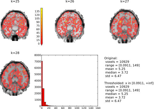
In interactive mode it is possible to click on the histogram to adjust the thresholding of the overlay volumes. Left-click sets the value corresponding to the lowest value in the colormap, and right-click set the value for the upper end of the colormap. Try right-clicking somewhere at the beginning of the x-axis and left on the end of the x-axis.

See also

The full source code of this example is included in the PyMVPA source distribution (doc/examples/mri_plot.py).