Classifying the MNIST handwritten digits with MDP¶

This example will demonstrate how to embed MDP‘s flows into a PyMVPA-based analysis. We will perform a classification of a large number of images of handwritten digits from the MNIST database. To get a better sense of how MDP blends into PyMVPA, we will do the same analysis with MDP only first, and then redo it in PyMVPA – only using particular bits from MDP.

But first we need some helper to load the MNIST data. The following function will load four NumPy arrays from an HDF5 file in the PyMVPA Data DB. These arrays are the digit images and the numerical labels for training and testing dataset respectively. All 28x28 pixel images are stored as flattened vectors.

import os
from mvpa2.base.hdf5 import h5load
from mvpa2 import pymvpa_datadbroot

def load_data():
    data = h5load(os.path.join(pymvpa_datadbroot, 'mnist', "mnist.hdf5"))
    traindata = data['train'].samples
    trainlabels = data['train'].sa.labels
    testdata = data['test'].samples
    testlabels = data['test'].sa.labels
    return traindata, trainlabels, testdata, testlabels

MDP-style classification¶

Here is how to get the classification of the digit images done in MDP. The data is preprocessed by whitening, followed by polynomial expansion, and a subsequent projection on a nine-dimensional discriminant analysis solution. There is absolutely no need to do this particular pre-processing, it is just done to show off some MDP features. The actual classification is performed by a Gaussian classifier. The training data needs to be fed in different ways to the individual nodes of the flow. The whitening needs only the images, polynomial expansion needs no training at all, and FDA as well as the classifier also need the labels. Moreover, a custom iterator is used to feed data in chunks to the last two nodes of the flow.

import numpy as np
import mdp

class DigitsIterator:
    def __init__(self, digits, labels):
        self.digits = digits
        self.targets = labels
    def __iter__(self):
        frac = 10
        ll = len(self.targets)
        for i in xrange(frac):
            yield self.digits[i*ll/frac:(i+1)*ll/frac], \
                  self.targets[i*ll/frac:(i+1)*ll/frac]

traindata, trainlabels, testdata, testlabels = load_data()

fdaclf = (mdp.nodes.WhiteningNode(output_dim=10, dtype='d') +
          mdp.nodes.PolynomialExpansionNode(2) +
          mdp.nodes.FDANode(output_dim=9) +
          mdp.nodes.GaussianClassifier())

fdaclf.verbose = True

fdaclf.train([[traindata],
               None,
               DigitsIterator(traindata,
                              trainlabels),
               DigitsIterator(traindata,
                              trainlabels)
               ])

After training, we feed the test data through the flow to obtain the predictions. First through the pre-processing nodes and then through the classifier, extracting the predicted labels only. Finally, the prediction error is computed.

feature_space = fdaclf[:-1](testdata)
guess = fdaclf[-1].label(feature_space)
err = 1 - np.mean(guess == testlabels)
print 'Test error:', err

Doing it the PyMVPA way¶

Analog to the previous approach we load the data first. This time, however, we convert it into a PyMVPA dataset. Training and testing data are initially created as two separate datasets, get tagged as ‘train’ and ‘test’ respectively, and are finally stacked into a single Dataset of 70000 images and their numerical labels.

import pylab as pl
from mvpa2.suite import *

traindata, trainlabels, testdata, testlabels = load_data()
train = dataset_wizard(
        traindata,
        targets=trainlabels,
        chunks='train')
test = dataset_wizard(
        testdata,
        targets=testlabels,
        chunks='test')
# merge the datasets into on
ds = vstack((train, test))
ds.init_origids('samples')

For this analysis we will use the exact same pre-processing as in the MDP code above, by using the same MDP nodes, in an MDP flow that is shortened only by the Gaussian classifier. The glue between these MDP nodes and PyMVPA is the MDPFlowMapper. This mapper is able to supply nodes with optional arguments for their training. In this example a DatasetAttributeExtractor is used to feed the labels of the training dataset to the FDA node (in addition to the training data itself).

fdaflow = (mdp.nodes.WhiteningNode(output_dim=10, dtype='d') +
           mdp.nodes.PolynomialExpansionNode(2) +
           mdp.nodes.FDANode(output_dim=9))
fdaflow.verbose = True

mapper = MDPFlowMapper(fdaflow,
                       ([], [], [DatasetAttributeExtractor('sa', 'targets')]))

The MDPFlowMapper can represent any MDP flow as a PyMVPA mapper. In this example, we attach the MDP-based pre-processing flow, wrapped in the mapper, to a classifier (arbitrarily chosen to be SMLR) via a MappedClassifier. In doing so we achieve that the training data is automatically pre-processed before it is used to train the classifier, and later on the same pre-processing it applied to the testing data, before the classifier is asked to make its predictions.

At last we wrap the MappedClassifier into a TransferMeasure that splits the dataset into a training and testing part. In this particular case this is not really necessary, as we could have left training and testing data separate in the first place, and could have called the classifier’s train() and predict() manually. However, when doing repeated train/test cycles as, for example, in a cross-validation this is not very useful. In this particular case the TransferMeasure computes a number of performance measures for us that we only need to extract.

tm = TransferMeasure(MappedClassifier(SMLR(), mapper),
                     Splitter('chunks', attr_values=['train', 'test']),
                     enable_ca=['stats', 'samples_error'])
tm(ds)
print 'Test error:', 1 - tm.ca.stats.stats['ACC']

Visualizing data and results¶

The analyses are already done. But for the sake of completeness we take a final look at both data and results. First and few examples of the training data.

examples = [3001 + 5940 * i for i in range(10)]

pl.figure(figsize=(2, 5))

for i, id_ in enumerate(examples):
    ax = pl.subplot(2, 5, i+1)
    ax.axison = False
    pl.imshow(traindata[id_].reshape(28, 28).T, cmap=pl.cm.gist_yarg,
             interpolation='nearest', aspect='equal')

pl.subplots_adjust(left=0, right=1, bottom=0, top=1,
                  wspace=0.05, hspace=0.05)
pl.draw()

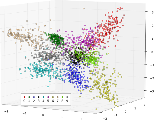
And finally we take a peak at the result of pre-processing for a number of example images for each digit. The following plot shows the training data on hand-picked three-dimensional subset of the original nine FDA dimension the data was projected on.

if externals.exists('matplotlib') \
   and externals.versions['matplotlib'] >= '0.99':
    from mpl_toolkits.mplot3d import Axes3D
    pts = []
    for i, ex in enumerate(examples):
        pts.append(mapper.forward(ds.samples[ex:ex+200])[:, :3])

    fig = pl.figure()

    ax = Axes3D(fig)
    colors = ('r','g','b','k','c','m','y','burlywood','chartreuse','gray')
    clouds = []
    for i, p in enumerate(pts):
        print i
        clouds.append(ax.plot(p[:, 0], p[:, 1], p[:, 2], 'o', c=colors[i],
                              label=str(i), alpha=0.6))

    ax.legend([str(i) for i in range(10)])
    pl.draw()