Curve-Fitting

Here we are going to take a look at a few examples of fitting a function to data. The first example shows how to fit an HRF model to noisy peristimulus time-series data.

First, importing the necessary pieces:

import numpy as np
from scipy.stats import norm

from mvpa2.support.pylab import pl
from mvpa2.misc.plot import plot_err_line, plot_bars
from mvpa2.misc.fx import *
from mvpa2 import cfg

BOLD-Response parameters

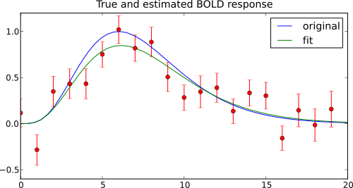
Let’s generate some noisy “trial time courses” from a simple gamma function (40 samples, 6s time-to-peak, 7s FWHM and no additional scaling:

a = np.asarray([single_gamma_hrf(np.arange(20), A=6, W=7, K=1)] * 40)
# get closer to reality with noise
a += np.random.normal(size=a.shape)

Fitting a gamma function to this data is easy (using resonable seeds for the parameter search (5s time-to-peak, 5s FWHM, and no scaling):

fpar, succ = least_sq_fit(single_gamma_hrf, [5,5,1], a)

With these parameters we can compute high-resultion curves for the estimated time course, and plot it together with the “true” time course, and the data:

x = np.linspace(0,20)
curves = [(x, single_gamma_hrf(x, 6, 7, 1)),
          (x, single_gamma_hrf(x, *fpar))]

# plot data (with error bars) and both curves
plot_err_line(a, curves=curves, linestyle='-')

# add legend to plot
pl.legend(('original', 'fit'))
pl.title('True and estimated BOLD response')

Searchlight accuracy distributions

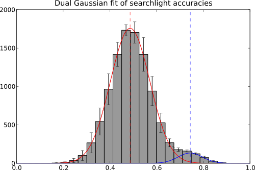
When doing a searchlight analysis one might have the idea that the resulting accuracies are actually sampled from two distributions: one causes by an actual signal source and the chance distribution. Let’s assume the these two distributions can be approximated by a Gaussian, and take a look at a toy example, how we could explore the data.

First, we generate us a few searchlight accuracy maps that might have been computed in the folds of a cross-validation procedure. We generate the data from two normal distributions. The majority of datapoints comes from the chance distribution that is centered at 0.5. A fraction of the data is samples from the “signal” distribution located around 0.75.

nfolds = 10
raw_data = np.vstack([np.concatenate((np.random.normal(0.5, 0.08, 10000),
                                      np.random.normal(0.75, 0.05, 500)))
                        for i in range(nfolds)])

Now we bin the data into one histogram per fold and fit a dual Gaussian (the sum of two Gaussians) to the total of 10 histograms.

histfit = fit2histogram(raw_data,
                        dual_gaussian, (1000, 0.5, 0.1, 1000, 0.8, 0.05),
                        nbins=20)
H, bin_left, bin_width, fit = histfit

All that is left to do is composing a figure – showing the accuracy histogram and its variation across folds, as well as the two estimated Gaussians.

# new figure
pl.figure()

# Gaussian parameters
params = fit[0]

# plot the histogram
plot_bars(H.T, xloc=bin_left, width=bin_width, yerr='std')

# show the Gaussians
x = np.linspace(0, 1, 100)
# first gaussian
pl.plot(x, params[0] * norm.pdf(x, params[1], params[2]), "r-", zorder=2)
pl.axvline(params[1], color='r', linestyle='--', alpha=0.6)
# second gaussian
pl.plot(x, params[3] * norm.pdf(x, params[4], params[5]), "b-", zorder=3)
pl.axvline(params[4], color='b', linestyle='--', alpha=0.6)
# dual gaussian
pl.plot(x, dual_gaussian(x, *params), "k--", alpha=0.5, zorder=1)
pl.xlim(0, 1)
pl.ylim(ymin=0)

pl.title('Dual Gaussian fit of searchlight accuracies')

And this is how it looks like.

See also

The full source code of this example is included in the PyMVPA source distribution (doc/examples/curvefitting.py).